10 Countability, Separation and Urysohn Metrization
· Denis Auroux
Countability axioms (§30)
Definition 10.1. is first-countable if , a countable basis of neighborhoods at , i.e. open such that every neighborhood contains one of the .
Example 10.2. Metric spaces are first-countable: at , take .
In a first-countable space, a sequence with . (Otherwise only holds.)
Definition 10.3. is second-countable if its topology has a countable basis.
Example 10.4. is second-countable, e.g. basis or .
with the product topology is second-countable (basis = products of a finite number of ,, where all remaining factors are ), while the uniform topology isn’t (because there exist uncountably many disjoint open subsets: the balls of radius centered at the points of ).
Second-countable a countable dense subset (e.g. take one point in each basis open set!). The converse holds for metric spaces (take balls of radius around points of the dense subset) but is false in general: is first-countable and has a countable dense subset, but a countable basis (so isn’t metrizable; HW4).
Regular and normal spaces (§31–32)
Recall: is Hausdorff := we can separate points: ,, disjoint open. (: is closed .)
Stronger separation axioms:
Definition 10.5. Suppose one-point subsets are closed (). Then say:
is regular if , closed disjoint from , disjoint open sets ,.
is normal if disjoint closed subsets, disjoint open sets ,.
(The first implication: will see.)
Example 10.6. is normal but not metrizable; is regular but not normal. See Munkres §31 for these and more.
Theorem 10.7.
regular + second-countable normal (won’t prove)
Hausdorff + compact normal (cf. HW2, Munkres 26.5)
Theorem 10.8. Metric spaces are normal.
Proof. Let be disjoint closed subsets of .
, such that ., such that . Let
(clearly open: unions of balls). We claim . Indeed, if then , such that . So
But this is a contradiction (e.g. if then !).∎
We can now ask which topological spaces are metrizable. We’ve seen: metrizable first-countable and normal (; counterexample: ).
Theorem 10.9 (Urysohn metrization theorem). If is regular and has a countable basis, then it is metrizable.
(The first condition is necessary; the second one is stronger than needed. The Nagata–Smirnov theorem gives a sharper criterion but is more technical to state and prove.)
Urysohn’s lemma
Urysohn’s lemma is the key ingredient in the proof of the metrization theorem.
Theorem 10.10 (Urysohn’s lemma). Let be a normal space and disjoint closed subsets. Then continuous such that and .
Idea:
Construct open sets such that , and moreover . Also set for .
Define , and show is continuous.
Step 1 uses the following reformulation of normality:
Lemma 10.11. is normal closed, open, open such that and . (In fact .)
Proof. and are disjoint closed sets, so since is normal, , open such that . Moreover, is closed and , so . So
∎
Proof of Urysohn’s lemma
Proof.Step 1. Given and disjoint closed, let , and let be open such that .
Next, we construct ,, such that , by induction. Choose a labelling of by an infinite sequence such that and (could e.g. continue: ).
Assuming have already been chosen, we construct using the above lemma: let
so and none of the rationals already considered lie in between. Then by the induction hypothesis, , hence using normality open such that ; let .
By induction, we construct in this way all the ’s, and indeed .
We also set if and if (still true: !).
Step 2. Define , where .
Since and , we have , so . Also, , and and .
So it only remains to show that is continuous! For this, observe:
: indeed, if then , so .
: indeed, if then .
Now given an open interval , we show is open in . Assume , and let such that .
By the above observation, and . So is open, and a neighborhood of . Moreover,
Hence , i.e. contains neighborhoods of its points. ∎
Proof of the metrization theorem
Now we prove the metrization theorem, namely that if is normal and has a countable basis, then is metrizable. We actually do this by embedding as a subspace of a metric space, namely with the product topology or the uniform topology; in fact both come from metrics.
For the product topology:
Key point: for this factor is all of .
Lemma 10.12 (Step 1). There exists a countable collection of continuous functions such that , neighborhood , such that and on .
Proof. This follows from Urysohn’s lemma, but we need to be careful so that countably many functions suffice.
Let be a countable basis for . If open, then such that . But then, since is normal, open such that , and such that , so that
So: for every such that , apply Urysohn’s lemma to get such that on and on . This countable collection of functions has the stated property. ∎
Lemma 10.13 (Step 2). The map
is an embedding, i.e. continuous, injective, and is homeomorphic to .
(So the topology on is defined by the metric , QED.)
Proof.
is continuous in the product topology because each component is continuous .
is injective, since
Finally, we must show that is a homeomorphism . Since is a continuous bijection , it only remains to prove: open is open.
For this, let be any open set, and . Then such that and outside of . Let
which is open in . Then (since , and ), hence , with open in . This is true (), so we conclude that is open.
Hence is a homeomorphism, and is homeomorphic to a metric space! ∎
Gluing and quotients (§22)
One good way to build interesting topological spaces is by “gluing” together simpler spaces.
Example 10.14.
The construction underlying this is the quotient topology.
Notes not reached in this lecture, covered at the start of Lecture 12
Definition 10.15. Let be a topological space, a set, a surjective map. The quotient topology on is defined by:
(Exercise: check this is a topology on , in fact the finest topology for which is continuous.)
Definition 10.16. A map between topological spaces is called a quotient map if is surjective and is open is open (i.e. the topology on is the quotient topology induced by ).
Typically, we start from an equivalence relation on , define to be the set of equivalence classes , and define ,. Conversely, given any surjective map , we can define an equivalence relation on by , and then .
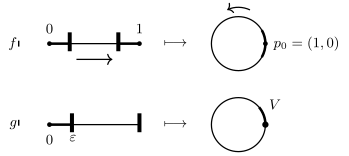
Example 10.17. with glued to : set , so is one equivalence class (all others are just ). The quotient map is
![Neighborhoods of 0 and 1 in [0,1] map to an arc around (1,0); for g on [0,1), the image of 0,epsilon) is not open
(Check! Away from the end points, is a homeomorphism , so we only need to check at and . The point is: open in open in .)
Versus: is not a quotient map! is not open in , versus open in ; we want iff!
Example 10.18. Let be topological spaces, each ; pick one point , and let be the quotient space of by the equivalence relation (glue the at their base points). This is called the wedge of the circles .
There is a useful characterization of continuous maps from a quotient space: if and is a map such that , then we can define by .
Theorem 10.19. If is a continuous map and , then, equipping with the quotient topology, is a continuous map.
Proof. Let , be the quotient map, and recall (independent of the choice of ). So . Hence: open, is open. By definition of the quotient topology ( open open), we conclude that is open. ∎
(And conversely, since is continuous. So: continuous continuous.)
Example 10.20.; define an equivalence relation iff lie on the same line through the origin, i.e. for some ,. This is an equivalence relation. The quotient space is projective -space, with the quotient topology (“the space of lines through in ”).
If is another topological space, then a continuous map is the same thing as a continuous map such that ,. (More about on the HW.)
Example 10.21 (Quotients of the unit square). Various quotients of the unit square : let the edges be ,,,.
(1) Gluing to by , we get a cylinder.
A neighborhood of a point on the gluing line corresponds to two neighborhoods of and in .
(2) If instead we glue to by , we get a Möbius band!
(3) Gluing to via and to by gives us the torus.
(4) Gluing and , however, gives the Klein bottle, which cannot be embedded in (we can draw a picture that self-intersects).